The Dirac delta function is a function introduced in 1930 by P. A. M. Dirac in his seminal book on quantum mechanics.[1] A physical model that visualizes a delta function is a mass distribution of finite total mass M—the integral over the mass distribution. When the distribution becomes smaller and smaller, while M is constant, the mass distribution shrinks to a point mass, which by definition has zero extent and yet has a finite-valued integral equal to total mass M. In the limit of a point mass the distribution becomes a Dirac delta function.
Heuristically, the Dirac delta function can be seen as an extension of the Kronecker delta from integral indices (elements of  ) to real indices (elements of
  ). Note that the Kronecker delta acts as a "filter" in a summation:
![{\displaystyle \sum _{i=m}^{n}\;f_{i}\;\delta _{ia}={\begin{cases}f_{a}&\quad {\hbox{if}}\quad a\in [m,n]\subset \mathbb {Z} \\0&\quad {\hbox{if}}\quad a\notin [m,n].\end{cases}}}](https://wikimedia.org/api/rest_v1/media/math/render/svg/d423840356e3321bcaf55a6694917325439011a7)
In analogy, the Dirac delta function δ(x−a) is defined by (replace i by x and the summation over i by an integration over x),
![{\displaystyle \int _{a_{0}}^{a_{1}}f(x)\delta (x-a)\mathrm {d} x={\begin{cases}f(a)&\quad {\hbox{if}}\quad a\in [a_{0},a_{1}]\subset \mathbb {R} ,\\0&\quad {\hbox{if}}\quad a\notin [a_{0},a_{1}].\end{cases}}}](https://wikimedia.org/api/rest_v1/media/math/render/svg/afb48bb90df31264053453233a5fcd22dba38ea8)
The Dirac delta function is not an ordinary well-behaved map  , but a distribution, also known as an improper or generalized function. Physicists express its special character by stating that the Dirac delta function only makes sense as a factor in an integrand ("under the integral"). Mathematicians say that the delta function is a linear functional on a space of test functions.
Properties
Most commonly one takes the lower and the upper bound in the definition of the delta function equal to  and
and  , respectively. From here on this will be done.

The physicist's proof of these properties proceeds by making proper substitutions into the integral and using the ordinary rules of integral calculus. The delta function as a Fourier transform of the unit function f(x) = 1 (the second property) will be proved below.
The last property is the analogy of the multiplication of two identity matrices,

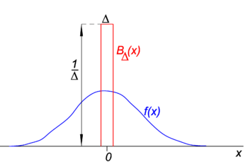
CC Image Fig. 1. Block ("boxcar") function (red) times regular function
f(
x) (blue).
Delta-convergent sequences
There exist families of regular functions Fα(x) of which the family members differ by the value of a single parameter α. An example of such a family is formed by the family of Gaussian functions Fα(x) = exp(−αx²), where the different values of the single parameter α distinguish the different members. When all members are linearly normalizable, i.e., the following integral is finite irrespective of α,

and all members peak around x = 0, then the family may form a delta-convergent sequence.
Block functions
The simplest example of a delta-convergent sequence is formed by the family of block functions, characterized by positive Δ,

In Fig. 1 the block function BΔ is shown in red. Evidently, the area (width times height) under the red curve is equal to unity, irrespective of the value of Δ,

Let the arbitrary function f(x) (blue in Fig. 1) be continuous (no jumps) and finite in the neighborhood of x=0. When Δ becomes very small, and the block function very narrow (and necessarily very high because width times height is constant) the product f(x) BΔ(x) becomes in good approximation equal to f(0) BΔ(x). The narrower the block the better the approximation. Hence for Δ going to zero,

which may be compared with the definition of the delta function,

This shows that the family of block functions converges to the Dirac delta function for decreasing parameter Δ; the family forms a delta-convergent sequence:


CC Image Fig. 2. Gaussian functions.
Note: We integrated over the whole real axis. Obviously this is not necessary, we could have excluded the zero-valued wings of the block function and integrated only over the hump in the middle, from −Δ/2 to +Δ/2. In mathematical texts, as e.g. Ref. [2], this refinement in the integration limits is included in the definition of the delta-convergent sequence. That is, it is required that the integrals over the two wings vanish in the limit. Because the delta-convergent sequences encountered in physical applications usually satisfy this condition, we omit the more exact mathematical definition.
Gaussian functions
Consider the family,

As is shown in Fig. 2 the functions peak around x = 0 and become narrower for decreasing α. Hence the family of Gaussian functions forms a delta-convergent sequence,

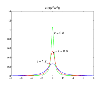
CC Image Fig. 3. Lorentz-Cauchy functions
Lorentz-Cauchy functions
The family of functions shown in Fig. 3

forms a delta-convergent sequence,

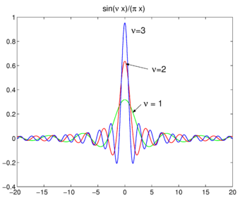
CC Image Fig. 4. Sinc functions.
Sinc functions
The family of functions (often called sinc functions) shown in Fig. 4 is

This family converges to the delta function for increasing ν

This limit leads readily to the Fourier integral representation of the delta function:
![{\displaystyle \int _{-\nu }^{\nu }e^{ikx}\mathrm {d} k={\frac {1}{ix}}\left[e^{ikx}\right]_{-\nu }^{\nu }={\frac {2\sin \nu x}{x}},}](https://wikimedia.org/api/rest_v1/media/math/render/svg/4ed1b5d539831626ce985ec41f4587d65223b5d6)
so that

The Dirac delta function is the Fourier transform of the unit function f(x) = 1.
Derivatives of the delta function
Consider a differentiable function f(x) that vanishes at plus and minus infinity. Integrate by parts

In the same way as one proves the turnover rule and Hermiticity of the quantum mechanical momentum operator  , we showed here that d/dx is anti-Hermitian,

Indeed, when we write the integral as an inner product, it follows from partial integration and the vanishing of f(x) on the integration limits that

This turnover rule is used as the definition of the derivative of the delta function,

where the prime indicates the first derivative of f(x). According to the definition of the delta function the first derivative is evaluated in x = 0. Using m times the turnover rule, it follows that the mth derivative of the delta function is defined by

Properties of the derivative

These results can be proved by making the substitution x → −x and use of the turnover rule for d/dx (see above).
Primitive
As shown here the primitive (also known as antiderivative, or undetermined integral) of the Dirac delta is the Heaviside step function H(x),

Clearly,

The Dirac delta function in three dimensions
Write the delta function in three-dimensional space as δ(r), with r = (x,y, z), and define,

From which follows more generally,

The three-dimensional delta function can be factorized

In spherical polar coordinates

Proof of equation (1)
Write

The Jacobian (Jacobi determinant) of this transformation from Cartesian coordinates to spherical polar coordinates is

Consider

so that

and

The last line in equation (1) follows from the chain rule.
The following useful and frequently applied property is proved [[Green's_function#Proof of Green function of ∇sup>2|here]],

where ∇2 is the Laplace operator in three-dimensional Cartesian coordinates and r is the length of r.
References
- ↑ P. A. M. Dirac, The Principles of Quantum Mechanics, Oxford University Press (1930). Fourth edition 1958. Paperback 1981, p. 58
- ↑ I. M. Gel'fand and G. E. Shilov, Generalized Functions, vol. 1, Academic Press, New York (1964). Translated from the Russian by E. Saletan.
- A. Messiah, Quantum Mechanics, vol. I. North Holland, Amsterdam (1967), Appendix A
- C. Cohen-Tannoudji, B. Diu, and F. Laloë, Quantum Mechanics, John Wiley, New York, (1977), Vol. 2, Appendix B.


