Point-normal representation
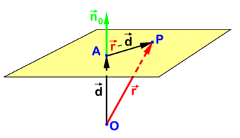
PD Image Fig. 1. Equation for plane. P is arbitary point in plane;
and
are collinear.
In analytic geometry several closely related algebraic equations are known for a plane in three-dimensional Euclidean space. One such equation is illustrated in figure 1. Point P is an arbitrary point in the plane and O (the origin) is outside the plane. The point A in the plane is chosen such that vector
![{\displaystyle {\vec {d}}\equiv {\overrightarrow {OA}}}](https://wikimedia.org/api/rest_v1/media/math/render/svg/e36e2b3dc5fa9a5197f9893441a4d25e86c6b93c)
is orthogonal to the plane. The collinear vector
![{\displaystyle {\vec {n}}_{0}\equiv {\frac {1}{d}}{\vec {d}}\quad {\hbox{with}}\quad d\equiv \left|{\vec {d}}\,\right|}](https://wikimedia.org/api/rest_v1/media/math/render/svg/7a7618570d19e424b5ccd749b18cae10c4371922)
is a unit (length 1) vector normal (perpendicular) to the plane which is known as the normal of the plane in point A. Note that d is the distance of O to the plane. The following relation holds for an arbitrary point P in the plane
![{\displaystyle \left({\vec {r}}-{\vec {d}}\;\right)\cdot {\vec {n}}_{0}=0\quad {\hbox{with}}\quad {\vec {r}}\equiv {\overrightarrow {OP}}\quad {\hbox{and}}\quad {\vec {r}}-{\vec {d}}={\overrightarrow {AP}}.}](https://wikimedia.org/api/rest_v1/media/math/render/svg/cb0fff5fff9086e57152477a370256bde96a5c85)
This equation for the plane can be rewritten in terms of coordinates with respect to a Cartesian frame with origin in O. Dropping arrows for component vectors (real triplets) that are written bold, we find
![{\displaystyle \left(\mathbf {r} -\mathbf {d} \right)\cdot \mathbf {n} _{0}=0\Longleftrightarrow xa_{0}+yb_{0}+zc_{0}=d}](https://wikimedia.org/api/rest_v1/media/math/render/svg/3d37bdf09641d6244e5f46505c76e06955934181)
with
![{\displaystyle \mathbf {d} =(a,\;b,\;c),\quad \mathbf {n} _{0}=(a_{0},\;b_{0},\;c_{0}),\quad \mathbf {r} =(x,\;y,\;z),}](https://wikimedia.org/api/rest_v1/media/math/render/svg/9795ec78f4905c32c8838372d2b23b017b6be2aa)
and
![{\displaystyle \mathbf {d} \cdot \mathbf {n} _{0}={\frac {1}{d}}\mathbf {d} \cdot \mathbf {d} =d={\sqrt {a^{2}+b^{2}+c^{2}}}.}](https://wikimedia.org/api/rest_v1/media/math/render/svg/f8561f6154d6c3187ff09f5923e8695531bef1b7)
Conversely, given the following equation for a plane
![{\displaystyle ax+by+cz=e,\,}](https://wikimedia.org/api/rest_v1/media/math/render/svg/1a29e27177c9158decab6630e79da7a59ce69b14)
it is easy to derive the same equation.
Write
![{\displaystyle \mathbf {r} =(x,\;y,\;z),\quad \mathbf {f} =(a,\;b,\;c),\quad {\hbox{and}}\quad \mathbf {d} \equiv \left({\frac {e}{a^{2}+b^{2}+c^{2}}}\right)\mathbf {f} .}](https://wikimedia.org/api/rest_v1/media/math/render/svg/7bd6bde0291ba8fd745dd5e817aa0284c087bfd7)
It follows that
![{\displaystyle \mathbf {f} \cdot \mathbf {r} =e=\mathbf {f} \cdot \mathbf {d} .}](https://wikimedia.org/api/rest_v1/media/math/render/svg/f68855edc01b123d5f3955fdf254dcb50d4d0bce)
Hence we find the same equation,
![{\displaystyle \mathbf {f} \cdot (\mathbf {r} -\mathbf {d} )=0\;\Longrightarrow \;(\mathbf {r} -\mathbf {d} )\cdot \mathbf {n} _{0}=0\quad {\hbox{with}}\quad \mathbf {n} _{0}={\frac {1}{\sqrt {a^{2}+b^{2}+c^{2}}}}\mathbf {f} }](https://wikimedia.org/api/rest_v1/media/math/render/svg/cf4ed176eb8568ce408fdbd68872ef0d739f19a5)
where f , d, and n0 are collinear. The equation may also be written in the following mnemonically convenient form
![{\displaystyle \mathbf {d} \cdot (\mathbf {r} -\mathbf {d} )=0,}](https://wikimedia.org/api/rest_v1/media/math/render/svg/55fc00923067395b6e403232526b3a0045b038f7)
which is the equation for a plane through a point A perpendicular to
.
Three-point representation
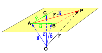
PD Image Fig. 2. Plane through points A, B, and C.
Figure 2 shows a plane that by definition passes through non-coinciding points A, B, and C that moreover are not on one line. The point P is an arbitrary point in the plane and the reference point O is outside the plane. Referring to figure 2 we introduce the following definitions
![{\displaystyle {\vec {a}}={\overrightarrow {OA}},\quad {\vec {b}}={\overrightarrow {OB}},\quad {\vec {c}}={\overrightarrow {OC}},\quad {\vec {r}}={\overrightarrow {OP}}.}](https://wikimedia.org/api/rest_v1/media/math/render/svg/6d214c29188e3f29c0e397ab8b19f17eb3528339)
Clearly the following two non-collinear vectors belong to the plane
![{\displaystyle {\vec {u}}={\overrightarrow {AB}}={\vec {b}}-{\vec {a}},\quad {\vec {v}}={\overrightarrow {AC}}={\vec {c}}-{\vec {a}}.}](https://wikimedia.org/api/rest_v1/media/math/render/svg/c56b5d74eb9745570dea51add05b94bcb2ef7f4b)
Because a plane (an affine space), with a given fixed point as origin is a 2-dimensional linear space and two non-collinear vectors with "tails" in the origin are linearly independent, it follows that any vector in the plane can be written as a linear combination of these two non-collinear vectors (this is also expressed as: any vector in the plane can be decomposed into components along the two non-collinear vectors). In particular, taking A as origin in the plane,
![{\displaystyle {\overrightarrow {AP}}={\vec {r}}-{\vec {a}}=\lambda {\vec {u}}+\mu {\vec {v}},\qquad \lambda ,\mu \in \mathbb {R} .}](https://wikimedia.org/api/rest_v1/media/math/render/svg/607871a3fcd6c995093be375274d01e312457a06)
The real numbers λ and μ specify the direction of
. Hence the following equation for the position vector
of the arbitrary point P in the plane:
![{\displaystyle {\vec {r}}={\vec {a}}+\lambda {\vec {u}}+\mu {\vec {v}}}](https://wikimedia.org/api/rest_v1/media/math/render/svg/5435eccd9463c6534cff707ebbc4ecd686bb92ea)
is known as the point-direction representation of the plane. This representation is equal to the three-point representation
![{\displaystyle {\vec {r}}={\vec {a}}+\lambda ({\vec {b}}-{\vec {a}})+\mu ({\vec {c}}-{\vec {a}}),}](https://wikimedia.org/api/rest_v1/media/math/render/svg/15671a6645c4d65c6ab75c600c71d295975d676d)
where
,
, and
are the position vectors of the three points that define the plane.
Writing for the position vector of the arbitrary point P in the plane
![{\displaystyle {\vec {r}}=(1-\lambda -\mu )\,{\vec {a}}+\lambda \,{\vec {b}}+\mu \,{\vec {c}}\;\equiv \;\xi _{1}\,{\vec {a}}+\xi _{2}\,{\vec {b}}+\xi _{3}\,{\vec {c}}\;,}](https://wikimedia.org/api/rest_v1/media/math/render/svg/38f91ae3e109c67c0291817df7df32e419cf9e27)
we find that the real triplet (ξ1, ξ2, ξ3) with ξ1 + ξ1 + ξ1 = 1 forms a set of coordinates for P. The numbers {ξ1, ξ2, ξ3 | ξ1+ ξ2+ ξ3 = 1 } are known as the barycentric coordinates of P. It is trivial to go from barycentric coordinates to the "three-point representation",
![{\displaystyle {\vec {r}}=\xi _{1}{\vec {a}}+\xi _{2}{\vec {b}}+\xi _{3}{\vec {c}}\quad {\hbox{with}}\quad \xi _{1}=1-\xi _{2}-\xi _{3}\;\Longleftrightarrow \;{\vec {r}}={\vec {a}}+\xi _{2}({\vec {b}}-{\vec {a}})+\xi _{3}({\vec {c}}-{\vec {a}}).}](https://wikimedia.org/api/rest_v1/media/math/render/svg/700b6bfec91099307adb46b80b18b5dc6cd4c10c)